3 Extremes, non-stationarity and climate change
One of the major impacts of climate change is a change in the amplitude and frequency of extreme weather conditions, including the intensification of extreme precipitation.
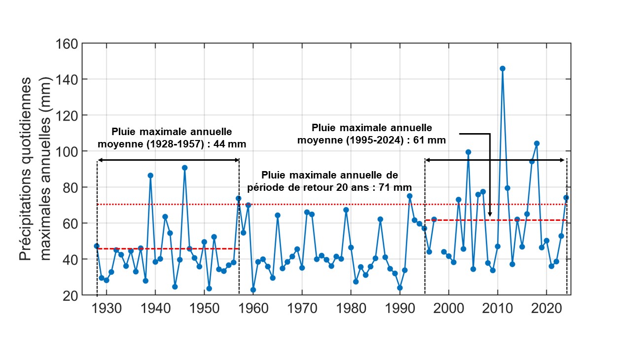
Let’s return to the example in Figure 2.1 to illustrate how climate change manifests. Beyond the large interannual variability, annual maximum precipitation appears to be increasing over time. The average over the first 30 years (1928–1957) was 44 mm, while the average for the last 30 years (1995–2024) was 61 mm (Figure 3.1). Applying a statistical test (the Mann-Kendall test at a 95% confidence interval; see Fact Sheet 6) confirms the hypothesis of an upward trend at this station (p-value < 0.01). This means that the trend is statistically significant. The estimated rate of change in extreme precipitation at the Chelsea station is 3.5% per decade.1 Such a series is said to be non-stationary.
The trend shown in Figure 3.1 is representative of the trends sometimes observed and generally simulated by climate models: a progressive increase or decrease in the average. It implies that the probability of observing an extreme value above certain thresholds increases over time. Look at the series in Figure 3.1 and consider the year 2000. The maximum annual precipitation with a 20-year return period2 could be estimated from the series available at that time (1928-2000), which was 71 mm.3 For the purposes of the example, imagine if this value were used in the design of a structure with the capacity to evacuate the runoff from 71 mm of rainfall. The capacity is likely to be exceeded, with the associated potential service disruptions, every 20 years on average. This threshold might be considered reasonable, depending on the designer’s risk tolerance. However, if we look at the values for the period from 2001 to 2024, we see that its capacity would have been exceeded nine years4 during this period, while only four years with exceedances occurred between 1928 and 2000. The risk during the 2001–2024 period goes well beyond what was initially established on the basis of the “historical” series. This example shows the importance of integrating climate change into designs.
The rate of change of the annual maximum precipitation was estimated using the Sen’s slope, also called the Theil–Sen estimator.↩︎
The return period is the average number of years between two consecutive years when this amount of rainfall occurred. The annual probability of exceedance (p) corresponding to a return period (T) is p = 1/T.↩︎
This value was obtained after fitting the Gumbel distribution to the data from 1928 to 2000 (see Fact Sheet 7).↩︎
It’s assumed that the capacity is exceeded only once a year, but that doesn’t mean that it can’t be exceeded more than once in a given year.↩︎