7 The statistical distribution of extreme values and the Gumbel distribution
The probabilities of the occurrence of the extreme values in a stationary random series are often represented by the Gumbel distribution, which is a particular case1 of the generalized extreme value distribution2. The Gumbel distribution is used by Environment and Climate Change Canada (ECCC) in the construction of Intensity-Duration-Frequency (IDF) curves3, among other things. The probability density function4 of the Gumbel distribution, \(f_{G}\left( x \right)\), is as follows: \[ f_{G}(x) = \sigma^{-1} z \exp(-z) \] with: \[ z = \exp \left[ \frac{-(x - \mu)}{\sigma} \right] \] where \(\mu\) is the position parameter and \(\sigma\) the scale parameter of the distribution.5 The corresponding distribution function6 is given by: \[ F_{G}(x) = \exp(-z) \] The method of moments7 can be used to estimate the Gumbel distribution parameters for a given series. If \(\overline{x}\) and s are the mean and standard deviation of the series, then the position parameters \(\hat{\mu}\) and the scale parameters \(\hat{\sigma}\) of the Gumbel distribution fitted to this series are obtained from the following expressions: \[ \begin{align} \widehat{\sigma} &= \sqrt{6} \left( \frac{s}{\pi} \right) \\ \widehat{\mu} &= \overline{x} - \frac{\sqrt{6} \gamma s}{\pi} \end{align} \] where \(\gamma\) is the Euler-Mascheroni constant (\(\gamma \approx 0.5772\)). Lastly, we can estimate a quantile for a given return period T (in years) by inverting the distribution function \(F\): \[ X = \widehat{\mu} - \widehat{\sigma} \ln \left[ - \ln \left( 1 - \frac{1}{T} \right) \right] \]
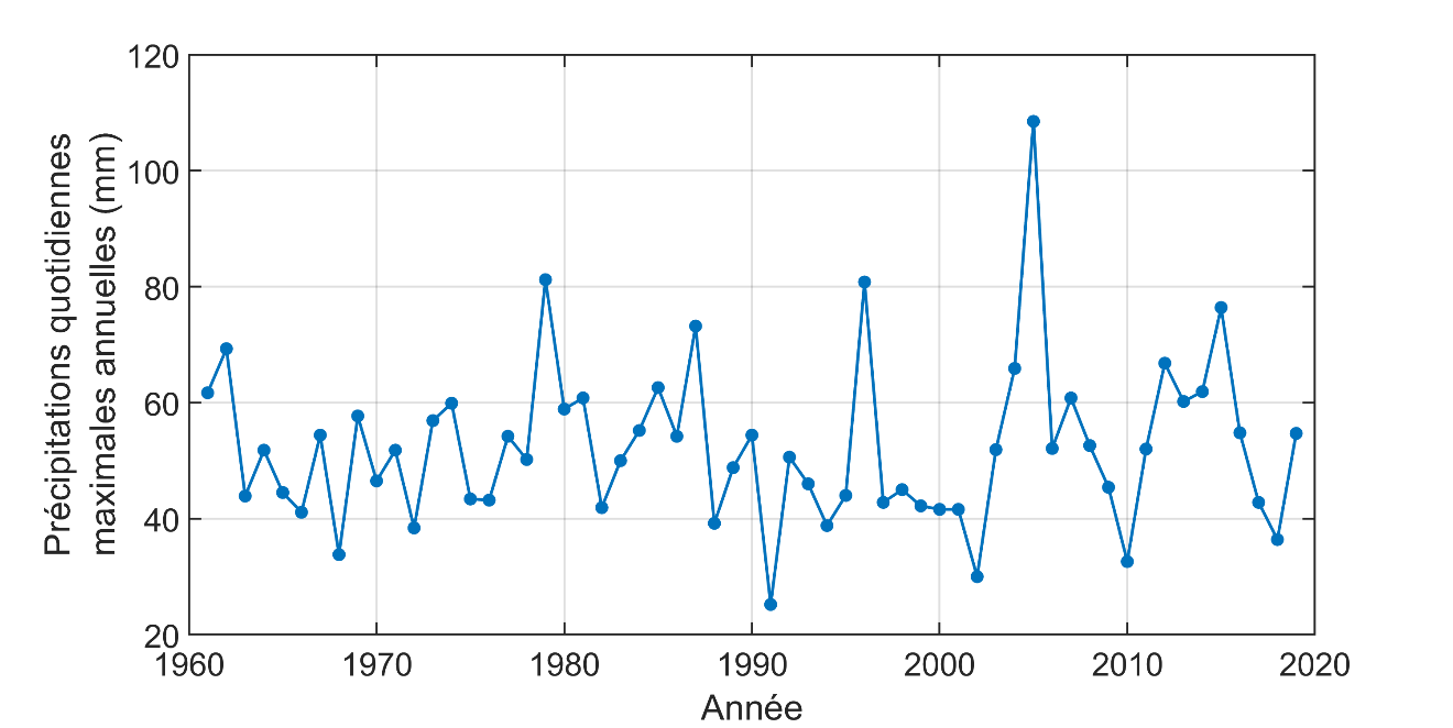
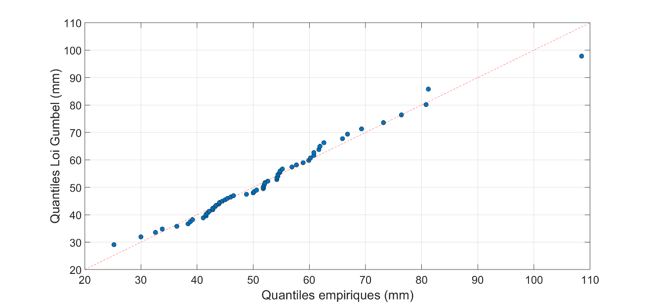
The Gumbel distribution was fitted to the values of the series of annual maximum daily precipitation values at the Jean-Lesage Airport8 station in Quebec (Figure 7.1). The values of the position and scale parameters after fitting are \(\hat{\mu} = 46.1\) and \(\hat{\sigma} = 10.9\). A quantile-quantile plot9 comparing quantiles estimated from the Gumbel distribution to empirical quantiles10 is shown in Figure 7.2. It can be seen that the agreement between the empirical quantiles and those of the Gumbel distribution is satisfactory and, therefore, one can conclude that the fitted Gumbel distribution adequately represents the series of annual daily precipitation maxima at the Jean-Lesage Airport station.
The Gumbel distribution corresponds to the case where the shape parameter of the generalized extreme value distribution is set to zero.↩︎
The use of the Gumbel distribution and the generalized extreme value distribution is based on theoretical considerations. Readers who want more details can consult Coles (2001).↩︎
For more details, see Engineering Climate Datasets.↩︎
The probability density function \(f(x)\) defines the probability that the value x is equal to a given value. Thus, \(f(x)\) dx is the probability that x is included in the interval \([x,x + dx]\).↩︎
The mean of the Gumbel distribution is \(\mu + \sigma\gamma\) where \(\gamma\) is the Euler-Mascheroni constant (\(\gamma \approx 0,5772\) and the variance is given by \(\frac{\pi^{2}\sigma^{2}}{6}\).↩︎
The cumulative distribution function \(F\left( x \right)\) defines the probability that the variable X is less than the value x, i.e. \(P\left( X < x \right) = F\left( x \right)\).↩︎
Several other estimation methods exist and have certain advantages over the method of moments (e.g. maximum likelihood estimation or the L-moment method). The method of moments is the one used by ECCC to create IDF curves in Canada.↩︎
The Jean-Lesage Airport station (7016294-701S001) is operated by Environment and Climate Change Canada.↩︎
Quantile-quantile plots compare the quantiles estimated from the distribution fitted to the data with the corresponding empirical quantiles.↩︎
The empirical quantiles were estimated using the Cunnane quantile estimator.↩︎